The Economic Factor Model and a class of affine term structure models

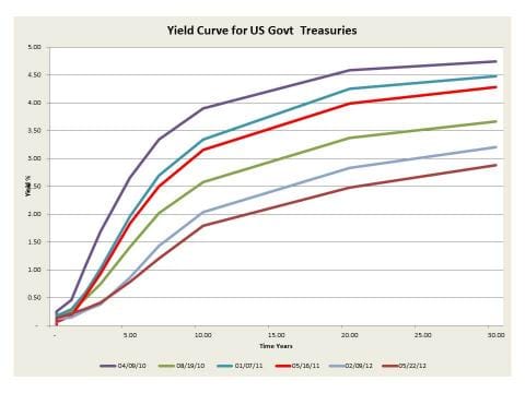
The economic factor model is an affine term structure model where the factors have a particular economic interpretation. The general affine n-factor term structure model is presented and the EFM as a special case is developed in detail. The results include general expressions for dynamics bond prices, forward curves and expected excess returns and risk premia.
For the special case EFM(2) the numerical calculations are presented in detail. A section on the Ornstein-Uhlenbeck process collects all the necessary results.
Click here for the full text.
The general n-factor Gaussian model
Notation
Matrix notation is used throughout. Primes$ ^\prime$ denote transpose. The vector $e_i\in\mathbb{R}^n$ is Cartesian basis vector $i$. Objective measure is $P$ and risk-neutral measure is $P^\star$. In order to avoid clutter the stars$ ^\star$ are occasionally dropped. Although this is always indicated: be careful.
Bond prices
Consider the general Gaussian real-world n-factor model under objective
measure
$$P:\quad d\xi = (A\xi+a),d t + \Sigma,d W, , A\in\mathbb{R}^{n\times n}, a\in\mathbb{R}^n \quad .$$
Via Girsanov transform to risk-neutral measure $P^\star$ with $d W = \lambda(\xi) d t+ d W^\star$ and $\lambda(\xi)$ affine we get:
$$\lambda(\xi)=\Sigma-(\Lambda\xi+\lambda1), , \Lambda\in\mathbb{R}^{n\times n}\quad .$$
Introducing $A^\star=A+\Lambda$ and $a\star=a+\lambda1$ leads to risk neutral dynamics
$$P^\star:\quad d\xi = (A\star\xi+a\star),d t + \Sigma,d W^\star \quad ,$$
The price $p(\tau,T)$ of a T-Bond (i.e. a zero-bond of maturity $T$) at time $\tau$ then satisfies the PDE
$$-r p + \frac{\partial p}{\partial\tau} + \left(\frac{\partial p}{\partial\xi}\right)^\prime (a\star+A\star\xi)+
{1\over 2}:\textsf{tr}:\Sigma^\prime \left(\frac{\partial^2 p}{\partial \xi\partial \xi}\right) \Sigma = 0.$$
Setting $t=T-\tau$ the ansatz $p(\tau,T) = p(t) = \exp\left(-u(t)^\prime\xi + v(t)\right)$ leads to the following two ODEs
$$\frac{\partial u}{\partial t} - {A\star}\prime u = (1,0,0)^\prime $$
$$\frac{\partial v}{\partial t} = -u^\prime a^\star + {1\over 2} u^\prime V u \qquad ,$$
with initial conditions $u(0) = 0$ and $v(0)=0$. The function $u(t)$ has a natural interpretation as duration with respect to the rates $\xi$, since $\partial\ln(P)/\partial\xi = u$. The solutions to the two ODEs are ...
Click here for the full text.
- Properties of the term structure
- $y(\infty)$ and $y(0)$
- Slope of the short end
-Instantaneous covariances - Unconditional finite-time yield dynamics
- Conditional finite-time yield dynamics ###
- The forward curve
- Expected excess returns and risk premier
- Bond portfolios
- Local efficient frontier
- Finite time portfolio evolution
- Sensitivity of prices and yields to volatilities
- Partial yield curve inversion using linearity in some parameters
- Sensitivity of yields to constant risk premia
EFM(2)
Click here for the full text.
- Introduction
- Model specification
- Diagonalisation of ${A\star}\prime$ and $A$
- Special results for EFM(2)
- u(t)
- $y(\infty)$
- $\mu_\infty$
OU-processes
Click here for the full text.
- Momenta
- OU-process in VAR form
- Maximum likelihood estimation
- Autocorrelation function and power spectrum
- Short observation times
- Estimation of OU processes
- Unrestricted estimation
- Restricted estimation
- Non-stationary OU-processes
Diagonalisation of outer product matrices
Click here for the full text.
Model specification - EFM(1)
Click here for the full text.


