The forward curve

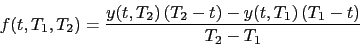
The forward rate $f(t,T_1,T_2)$ at time $t$ is defined as

$$f(t,T_1,T_2) = \frac{y(t,T_2)\,(T_2-t)-y(t,T_1)\,(T_1-t)}{T_2-T_1}$$ (20)

and the instantaneous forward rate $f(t,T)$ at time t is

$$f(t,T) = \lim_{T_1\to T_2} f(t,T_1,T_2) = \frac{\partial\left[(T-t)\,y(t,T)\right]}{\partial T} \quad .$$ (21)

Inserting the expression for $y(t,T)$ yields

$$f(t,T) = \frac{u^\prime(T-t)}{\partial T}\,\xi_t-\frac{\par... ...A^\star\,\xi + r + u^\prime a^\star - {1\over 2} u^\prime V u$$ (22)

where it is understood that $u=u(T-t)$, $\xi=\xi_t$, etc.

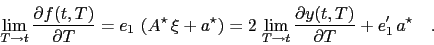
Short end slope The short end of the instantaneous forward curve is naturally related the short end of the zero curve, but also contains information about risk premia: Since 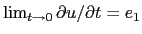$\lim_{t\to 0} \partial u/\partial t = e_1$ the short-end forward slope is

$$\lim_{T\to t}\frac{\partial f(t,T)}{\partial T} = e_1\,\lef... ...rac{\partial y(t,T)}{\partial T} + e_1^\prime\,a^\star\quad .$$ (23)