


Next: Bond prices under EFM(1)
Up: Model specification - EFM(1)
Previous: Model specification - EFM(1)
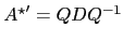
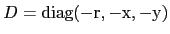
Eigenvalue decomposition of
 is possible for
  and
and  . Write
in short notation:
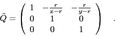
. Write
in short notation:
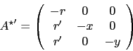 |
(101) |
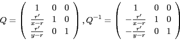
The eigenvalues are 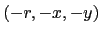 with eigenvectors (
 )
)
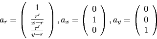 |
(102) |
The degenerate case  has eigenvectors
  ,
, ,
, .
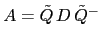
Then
.
Then
 with
with
 and
and
 |
(103) |
The inverse of
will be needed:
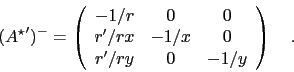 |
(104) |
Similarly
 with
with 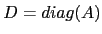 and
and
 |
(105) |
Markus Mayer
2009-06-22