Calculation of $\gamma$ and $\Omega$ : Sum-product derivation

Key to efficient calculation of any quantity in the HMM is the fact that the summations over hidden variables can be 'pulled' out. Rewrite the full joint eq. (2):

$$p(xs) = p(s_0) \prod_{t=1}^T \psi(x_t,s_t, s_{t-1}), \quad\mathrm{where}$$ (6)

$$\psi(s_t, s_{t-1},x_t,) = p(x_t\vert s_t)\,p(s_t\vert s_{t-1})$$ (7)

and the summations over the hidden variables $s_0\dots s_T$ can be regrouped

$$p(x) = \sum_{s}p(xs) = \sum_{s_T}\sum_{s_{T-1}} \psi(s_T,s_{T-1},x_T) \sum_{s_{T-2}} \psi(s_{T-1},s_{T-2},x_{T-1}) \times$$

$$\times\sum_{s_{T-3}}\dots\sum_{s_1} \psi(s_2,s_1,x_2) \sum_{s_0} \psi(s_1,s_0,x_1)\quad .$$

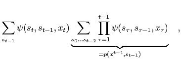
One term in the sequence of sums is

$$\sum_{s_{t-1}} \psi(s_t,s_{t-1},x_t) \underbrace{ \sum_{s_0\dots ... ...rod_{\tau=1}^{t-1} \psi(s_\tau,s_{\tau-1},x_\tau) }_{=p(x^{t-1},s_{t-1})}\quad,$$ (8)

so with the definition

$$\boxed{\alpha_t(s)=p(x^t,s_t=s)}$$ (9)

we obtain the forward recursion

$$\boxed{ \alpha_t(s) = \sum_{s^\prime} \psi(s,s^\prime,x_t) \alpha_{t-1}(s^\prime)\,, \quad\mathrm{with}\,\alpha_0(s) = 1\quad. }$$ (10)

Similarly, the summations for $p(x)$ can be arranged backward:

$$\sum_{s}p(xs) = \sum_{s_0}\sum_{s_1} \psi(s_1,s_0,x_1) \sum_{s_2} \psi(s_2,s_1,x_2) \sum_{s_3} \psi(s_3,s_2,x_3) \times$$

$$\times\sum_{s_4}\dots\sum_{s_T} \psi(s_T,s_{T-1},x_T)\quad .$$

With the introduction of

$$\boxed{\beta_t(s) := p(x_{t+1}\dots x_T\vert s_t=s)}$$ (11)

we obtain the backward recursion

$$\boxed{ \beta_t(s^\prime) = \sum_s \psi(s,s^\prime,x_{t+1})\,\beta_{t+1}(s)\,, \quad\mathrm{with}\,\beta_T(s^\prime) = 1\quad. }$$ (12)

Fig.: Graphical representation of $\alpha$

Fig.: Graphical representation of $\beta$

The desired quantities $\gamma_t(s)$ and $\Omega_t(s,s^\prime)$ defined in eq. (5) can be expressed in terms of $\alpha$ and $\beta$ . Observe that

$$p(x,s_t) = p(x^{[t+1}\vert s_t)\,p(x^ts_t) = \beta_t(s)\,\alpha_t(s)\,,\quad\mathrm{and}$$

$$p(x,s_{t-1},s_t) = \underbrace{p(x^{t-1},s_{t-1})}_{\alpha_{t-1}(s_{t-1})} \underbra... ..._t)}_{ \psi(s_t,s_{t-1},x_t) } \underbrace{p(x^{[t+1}\vert s_t)}_{\beta_t(s_t)}$$