Next: Analytical solutions for
Up: kelly
Previous: kelly
Let  be a real random variable with support
 . Following Kelly [1] consider the reinvested growth of a fixed fraction investment in an instrument that has payoff
.
. Following Kelly [1] consider the reinvested growth of a fixed fraction investment in an instrument that has payoff
.
(If the support of
is bounded the restriction on  can be relaxed.)
The long run growth rate is
can be relaxed.)
The long run growth rate is
By the law of large numbers
 |
(1) |
For a given
the function  is concave in
, and, writing
is concave in
, and, writing
 we have
 .
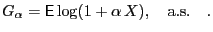
Define the maximal growth rate as
.
Define the maximal growth rate as
![$\displaystyle G[X] = \max_\alpha\,{\mathsf{E}}\log(1+\alpha\,X)\quad.$](img15.png) |
(2) |
![$ G[X]$](img16.png) and
and
 :
:
Since the slope of  at
at  , i.e.
, determines the location of the maximum we have, for
, i.e.
, determines the location of the maximum we have, for
![$ \alpha\in[0,1]$](img20.png) ,
,
Upper bound for
:
Jensen's inequality yields
 and because of
  and
and
 it is
it is
![$\displaystyle G[X] \leq \log(1+{\mathsf{E}}X) \leq {\mathsf{E}}X \quad .$](img29.png) |
(5) |
Mixtures:
Consider a mixture
 . We have
hence
![$\displaystyle G[X] \leq \max_Y G[X\vert Y] \quad ,$](img36.png) |
(6) |
i.e. the gain of a mixture cannot be larger than the gain of the best variable in the mixture.
Gambles that are offered with lower fequency  :
:
Suppose a gamble is offered at a reduced rate, i.e. at every step with probability
the payoff
is available and with probability  no investment is offered, i.e. the payoff is 0
. The pdf for payoff
no investment is offered, i.e. the payoff is 0
. The pdf for payoff  is
is
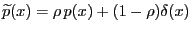 . Then
![$ \max_\alpha\widetilde{\mathsf{E}}\log(1+\alpha X) = \max_\alpha\left[\rho{\mathsf{E}}\log(1+\alpha X) + (1-\rho)\log(1)\right] = \rho G[X]$](img41.png) . Denoting the reduced rate gain, i.e. the maximal gain under
. Denoting the reduced rate gain, i.e. the maximal gain under
 , as
, as ![$ G^\rho[X]$](img43.png) , it is
, it is
![$\displaystyle G^\rho[X] = \rho\, G[X] \quad .$](img44.png) |
(7) |
When several gambles
 are offered with occurrence probabilities
 the individual gains are
![$ \rho_iG[X_i]$](img47.png) . Amongst the offered gambles the one with largest
is favourable.
. Amongst the offered gambles the one with largest
is favourable.
Small edge
 :
:
For small
we expand around
and the quadratic approximation gives
 and then
![$\displaystyle G[X] = \frac{1}{2} \frac{({\mathsf{E}}X)^2}{{\mathsf{E}}X^2},\quad \mathrm{for\ } {\mathsf{E}}X\rightarrow 0$](img51.png) |
(8) |
Gain of averages
 :
:
A lower bound to
![$ G[\sum_i w_i X_i]$](img53.png) with
with
 can easily be found:
By convexity of the  function it is
![$ \max_\alpha\sum_i w_i\,G_i(\alpha) \geq\sum_i w_i\, \max_\alpha G_i(\alpha) = \sum_i w_i G[X_i]$](img60.png) , so we have
, so we have
![$\displaystyle G\left[\sum_i w_i X_i\right] \geq \sum_i w_i G[X_i] \geq \min_i G[X_i] \quad$](img61.png) |
(9) |
i.e. the gain of an average of payoffs is not smaller than the smallest gain.
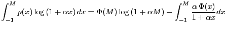
Representation in terms of the cumulative distribution function:
Partial integration of the integral
 results in a useful
representation for
. Denote the cdf
results in a useful
representation for
. Denote the cdf
 .
Starting with
.
Starting with
 partial integration gives (use
 )
)
observe that both terms separately diverge with
 . To alleviate this problem
use
. To alleviate this problem
use
 ,
,
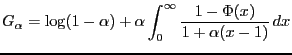
and after rearranging and letting
we have the desired result
 |
(10) |
Representation in terms of the Laplace transform:
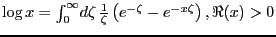
We will need a result for the Laplace transform of a (positive) random variable
,
 . Doing partial integration of
 analogous to the partial integration leading to
eq. (10) gives the following result that expresses the Laplace transform in terms of the cdf:
analogous to the partial integration leading to
eq. (10) gives the following result that expresses the Laplace transform in terms of the cdf:
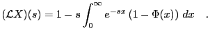 |
(11) |
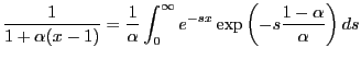
Starting with the shifted version of the cdf representation eq. (10)
and using
we get
and we can express the integral
 via eq. (11) in terms of the cdf
  to
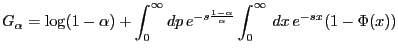
obtain
to
obtain
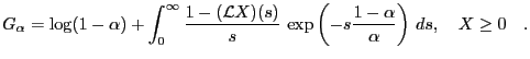 |
(12) |
The restriction  in the equation above is used as a reminder that the relation holds
for the unshifted, i.e. positive random variable
.
in the equation above is used as a reminder that the relation holds
for the unshifted, i.e. positive random variable
.
It is tempting to use
 to derive a relation, but issues with uniform continuity arise.
Next: Analytical solutions for
Up: kelly
Previous: kelly
Markus Mayer
2010-06-04
![$\displaystyle \max_\alpha{\mathsf{E}}_X\log(1+\alpha X) = \max_\alpha{\mathsf{E...
...mathsf{E}}_{X\vert Y}
\underbrace{\log(1+\alpha X\vert Y)}_{\leq G[X\vert Y]} =$](img33.png)
![$\displaystyle G\left[\sum_i w_i X_i\right]$](img55.png)
![$\displaystyle G_\alpha^M = \Phi(M)\left[\int_{-1}^M\frac{\alpha}{1+\alpha x} dx+\log(1-\alpha)\right] - \int_{-1}^M \frac{\alpha\,\Phi(x)} {1+\alpha x}\, dx$](img69.png)