


Next: Properties of the term
Up: The general -factor Gaussian
Previous: Notation
Bond prices
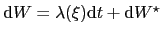
Consider the general Gaussian real-world n-factor model under objective measure
 |
(1) |
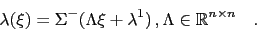
Via Girsanov transform to risk-neutral measure  with
with
 and
and  affine:
 |
(2) |
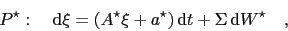
Introducing
 and
and
 leads to risk-neutral dynamics
 |
(3) |
The price  of a T-Bond (i.e. a zero-bond of maturity
  ) at time
  then satisfies the PDE
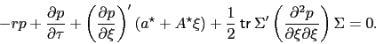 |
(4) |
Setting  the ansatz
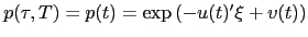 leads to the following two ODEs
with initial conditions  and
and  .
The function
.
The function  has a natural interpretation as duration with respect to the rates
  , since
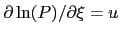 .
The solutions to the two ODEs are 1
.
The solutions to the two ODEs are 1
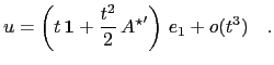
The asymptotics of  for
for  will be useful:
 |
|
|
(9) |
We turn to the calculation of and  via diagonalization of
 .
To avoid clutter the star
.
To avoid clutter the star will be dropped for the remainder of this subsection,
i.e. we write
will be dropped for the remainder of this subsection,
i.e. we write  for
for  , etc.
Assuming  can be diagonalised
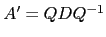 with diagonal
  the solution
may be rewritten
the solution
may be rewritten
where the following abbrevation was introduced:
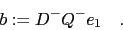 |
(10) |
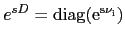
Denote the eigenvalues of by
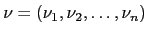 . Then
 and
and
 and
and
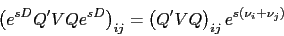 |
(11) |
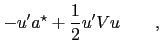
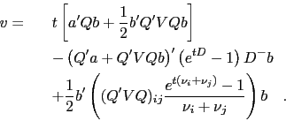
which makes integration towards straightforward:
This can be written in another form,
or, using the result for  from section
 ![[*]](crossref.png) below,
below,
Next: Properties of the term
Up: The general -factor Gaussian
Previous: Notation
Markus Mayer
2009-06-22

![$\displaystyle \int_0^t ds\left[-{a^\star}^\prime u + {1\over 2} u^\prime V u\right]\quad .$](img36.png)
![\begin{eqnarray*}
u &=& Q\left(e^{t D} -1\right) b\\
v &=& \int_0^t ds\left[a...
...\over 2} b^\prime e^{s D} Q^\prime V Q e^{s D} b\right] \quad ,
\end{eqnarray*}](img47.png)
![\begin{eqnarray*}
v = && a^\prime Q\left(t-\left(e^{tD}-1\right)D^-\right)b \\ ...
..._j)}-1}{\nu_i+\nu_j}-\frac{e^{t\nu_j}-1}{\nu_j}\right]\right) b
\end{eqnarray*}](img54.png)
![\begin{eqnarray*}
v = && -t\,y(\infty) + a^\prime Q\left(-\left(e^{tD}-1\right)...
...\nu_i+\nu_j}-\frac{e^{t\nu_j}-1}{\nu_j}\right]\right) b \quad .
\end{eqnarray*}](img56.png)